

Data Analysis with Pandas: Manipulating and Visualizing Data
Written by Yasin TANIŞ
Introduction
Data analysis has become an integral part of decision-making. Python stands out in this field thanks to its powerful libraries for analysing and manipulating data. One of them, pandas, is indispensable for data scientists because it is flexible and easy to use. In this article we look at the core features of pandas and how it is used in data analysis, with practical examples on real or synthetic data.
DataFrame and Series
Pandas works with two main data structures. A DataFrame is a two-dimensional structure of rows and columns. A Series is one-dimensional and represents a single column of data.
import pandas as pd

# Creating a simple DataFrame
data = {
    'name': ['Alice', 'Bob', 'Charlie'],
    'age': [25, 30, 35],
    'city': ['New York', 'Los Angeles', 'Chicago']
}
df = pd.DataFrame(data)
print(df)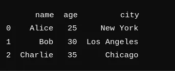
Creating DataFrames
There are many ways to create a DataFrame. You can load data from sources such as CSV, Excel and SQL and turn it into a DataFrame.
# Loading data from a CSV file
df = pd.read_csv('data.csv')

# Loading data from an Excel file
df = pd.read_excel('data.xlsx')

# Loading data from an SQL database
import sqlite3
conn = sqlite3.connect('database.db')
df = pd.read_sql_query('SELECT * FROM table', conn)
Loading and saving data
Pandas makes loading and saving data simple. You can read and process files in many different formats.
# Saving data
df.to_csv('new_data.csv', index=False)
df.to_excel('new_data.xlsx', index=False)
Cleaning and preparing data
Cleaning and preparation are critical steps in data analysis. Pandas makes it easy to handle missing values, convert data types and remove data you do not need.
# Checking for missing values
print(df.isnull().sum())

# Filling missing values
df.fillna(0, inplace=True)

# Converting data types
df['date'] = pd.to_datetime(df['date'])
Here we check whether the DataFrame has missing values. The output shows that none of the columns has any.
Statistical summaries
Pandas offers many tools for summarizing data quickly. Basic statistics and summaries are a single call away.
# Basic statistical summaries
print(df.describe())

# Summarizing specific columns
print(df['age'].mean())
print(df['age'].std())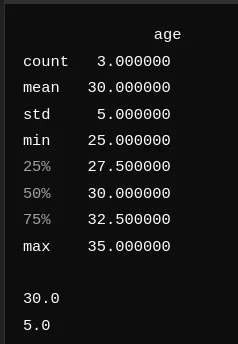
In the summary the mean age is 30 with a standard deviation of 5; the minimum and maximum ages are 25 and 35. This gives a quick picture of the age distribution in the data.
Grouping and summarizing
Grouping and summarizing is one of pandas' strengths. The groupby and pivot_table functions make it straightforward.
# Grouping and summarizing
group = df.groupby('city')['age'].mean()
print(group)

# Creating a pivot table
pivot = df.pivot_table(values='age', index='city', columns='gender', aggfunc='mean')
print(pivot)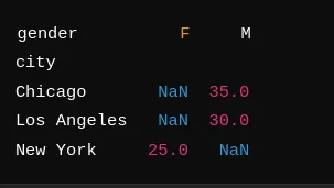
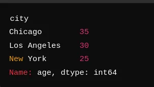
Grouping by city gives the average age for each one: Chicago (35), Los Angeles (30) and New York (25). The pivot table gives a similar summary broken down by gender; our example has no gender data, so those cells show NaN.
Visualizing data with pandas
Pandas has simple but effective plotting tools. Functions such as plot, hist and boxplot produce charts quickly.
# Basic plots
df['age'].plot(kind='hist')
df.plot(kind='scatter', x='age', y='income')
Working with Seaborn and Matplotlib
You can also visualize pandas data with Seaborn and Matplotlib, which allow more customized and detailed charts.
import seaborn as sns
import matplotlib.pyplot as plt

# Visualizing with Seaborn
sns.boxplot(x='city', y='age', data=df)
plt.show()
Time series analysis
Pandas handles time series data very well, which makes trends and patterns easy to find.
# Handling time series data
df['date'] = pd.to_datetime(df['date'])
df.set_index('date', inplace=True)
print(df.resample('M').mean())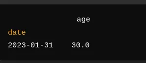
Here we convert the date column to datetime and set it as the index. Resampling by month and taking the mean gives an average age of 30 for January 2023.
Merging and combining data
Pandas has many functions for merging and combining data sets, such as merge, join and concat.
# Merging two DataFrames
df1 = pd.DataFrame({'name': ['Alice', 'Bob'], 'age': [25, 30]})
df2 = pd.DataFrame({'name': ['Alice', 'Bob'], 'city': ['New York', 'Los Angeles']})
merged_df = pd.merge(df1, df2, on='name')
print(merged_df)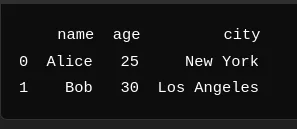
In this example we merge two DataFrames on the name column, combining each person's age and city.
Practical example: analysis with synthetic data
Creating the data
For a practical example we create synthetic data to show what pandas can do.
import pandas as pd
import numpy as np
import seaborn as sns
import matplotlib.pyplot as plt

# Creating synthetic data
np.random.seed(0)
dates = pd.date_range('20230101', periods=100)
df = pd.DataFrame(np.random.randn(100, 4), index=dates, columns=list('ABCD'))
df['Category'] = np.random.choice(['Category1', 'Category2', 'Category3'], size=100)
print(df.head())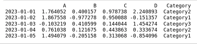
This creates a DataFrame of 100 rows with columns A, B, C and D and a categorical column Category. The values are random, and Category takes one of three values.
Analysis and visualization
With the synthetic data we run some basic analysis and draw charts.
# Statistical summary
print(df.describe())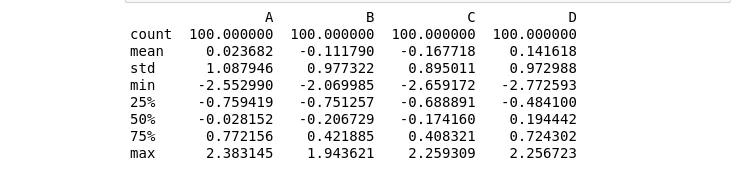
The summary gives a full overview of the data. The means of columns A, B, C and D are close to zero, as expected from a random normal distribution, and the standard deviations are close to 1, showing how widely the values spread around the mean.
# Grouping and summarizing
grouped = df.groupby('Category').mean()
print(grouped)
Grouping by Category shows the mean of each column for each category, which reveals how the categories differ.
# Visualizing data
df['A'].plot(kind='hist', title='Histogram of A')
plt.show()

sns.boxplot(x='Category', y='B', data=df)
plt.show()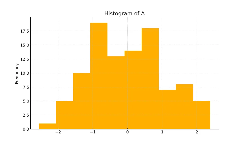
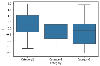
The histogram shows how the values in column A are distributed; the box plot shows column B across the categories. Charts like these help you understand the distribution and spot outliers or patterns.
Conclusion
Pandas is a versatile and powerful tool for data analysis; its flexibility and ease of use make it indispensable for data scientists. In this article we covered its core features and how they fit into an analysis, and we showed practical use on synthetic data. With further practice and more advanced techniques, you can go deeper into data science and draw more insight from your data with pandas.
References
- McKinney, W. (2010). Data Structures for Statistical Computing in Python. Proceedings of the 9th Python in Science Conference, 51–56.
- McKinney, W. (2017). Python for Data Analysis: Data Wrangling with Pandas, NumPy, and IPython (2nd ed.). O’Reilly Media.
- The pandas development team. pandas documentation. pandas.pydata.org
- NumPy documentation. numpy.org
- Matplotlib documentation. matplotlib.org
- Seaborn documentation. seaborn.pydata.org