

Python for Data Analysis: Matplotlib and Data Visualization
Written by Yasin TANIŞ

Introduction
Data visualization means using graphs and charts to make complex data sets easier to understand. Python offers several libraries for data analysis and visualization, and Matplotlib is one of the most popular. In this article we learn the basics of data visualization with Matplotlib.
What Matplotlib is
Matplotlib is a powerful, flexible library for creating 2D plots in Python. It can draw line charts, bar charts, scatter plots and many other kinds of plot.
Installing Matplotlib
Before using Matplotlib we need to install it. If it is not already on your system, install it with this command:
pip install matplotlibBasic usage
Let's start with a simple line plot.
import matplotlib.pyplot as plt
# Example data
x = [1, 2, 3, 4, 5]
y = [2, 3, 5, 7, 11]

# Creating a line plot
plt.plot(x, y)
plt.xlabel('X Axis')
plt.ylabel('Y Axis')
plt.title('Simple Line Plot')
plt.show()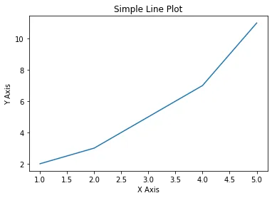
This simple example shows how to draw a line plot with Matplotlib. Now let's look at more plot types and customizations.
Types of plots
Bar charts
Bar charts are used to visualize categorical data.
import matplotlib.pyplot as plt

# Example data
categories = ['A', 'B', 'C', 'D', 'E']
values = [4, 7, 1, 8, 5]
# Creating a bar chart
plt.bar(categories, values)
plt.xlabel('Categories')
plt.ylabel('Values')
plt.title('Simple Bar Chart')
plt.show()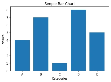
Scatter plots
Scatter plots show the relationship between two variables.
import matplotlib.pyplot as plt

# Example data
x = [5, 7, 8, 7, 2, 17, 2, 9, 4, 11]
y = [99, 86, 87, 88, 100, 86, 103, 87, 94, 78]
# Creating a scatter plot
plt.scatter(x, y)
plt.xlabel('X Variable')
plt.ylabel('Y Variable')
plt.title('Simple Scatter Plot')
plt.show()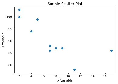
Histograms
Histograms show how data is distributed.
import matplotlib.pyplot as plt

# Example data
data = [1, 2, 2, 3, 3, 3, 4, 4, 4, 4, 5, 5, 5, 5, 5]
# Creating a histogram
plt.hist(data, bins=5)
plt.xlabel('Values')
plt.ylabel('Frequency')
plt.title('Simple Histogram')
plt.show()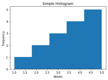
Pie charts
Pie charts show the proportions of categorical data.
import matplotlib.pyplot as plt
# Example data
labels = ['A', 'B', 'C', 'D']
sizes = [15, 30, 45, 10]
# Creating a pie chart
plt.pie(sizes, labels=labels, autopct='%1.1f%%', startangle=90)
plt.axis('equal')  # Equal aspect ratio ensures that pie is drawn as a circle.
plt.title('Simple Pie Chart')
plt.show()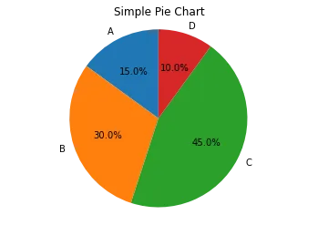
Customizing plots
Matplotlib lets you customize plots extensively so they are easier to read and more pleasing to look at.
Colours and styles
You can add colours and styles to make your plots more attractive.
import matplotlib.pyplot as plt

# Example data
x = [1, 2, 3, 4, 5]
y = [2, 3, 5, 7, 11]
# Customizing the line plot
plt.plot(x, y, color='red', linestyle='--', marker='o')
plt.xlabel('X Axis')
plt.ylabel('Y Axis')
plt.title('Customized Line Plot')
plt.show()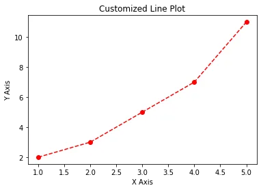
Plot size and resolution
You can adjust the size and resolution of a plot to fit different needs.
import matplotlib.pyplot as plt

# Example data
x = [1, 2, 3, 4, 5]
y = [2, 3, 5, 7, 11]
# Setting plot size and resolution
plt.figure(figsize=(10, 5), dpi=100)
plt.plot(x, y)
plt.xlabel('X Axis')
plt.ylabel('Y Axis')
plt.title('Large and High-Resolution Plot')
plt.show()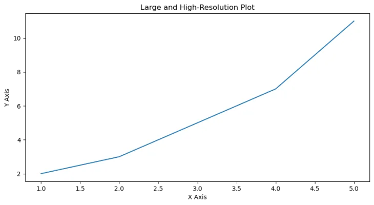
Subplots
Subplots let you draw several plots in a single figure.
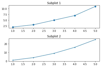
Logarithmic plots
Logarithmic plots are useful for data that spans a very wide range of values.
import matplotlib.pyplot as plt
import numpy as np

# Example data
x = np.linspace(0.1, 100, 100)
y = np.exp(x)
# Creating a logarithmic plot
plt.plot(x, y)
plt.xscale('log')
plt.yscale('log')
plt.xlabel('Log X Axis')
plt.ylabel('Log Y Axis')
plt.title('Logarithmic Plot')
plt.show()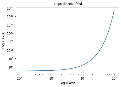
Advanced customization
Annotations
You can add annotations to highlight particular points.
import matplotlib.pyplot as plt

# Example data
x = [1, 2, 3, 4, 5]
y = [2, 3, 5, 7, 11]
# Creating a plot with annotation
plt.plot(x, y)
plt.annotate('Important Point', xy=(3, 5), xytext=(4, 10),
             arrowprops=dict(facecolor='black', shrink=0.05))
plt.xlabel('X Axis')
plt.ylabel('Y Axis')
plt.title('Annotated Plot')
plt.show()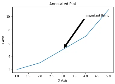
3D plots
Matplotlib can also draw 3D plots.
from mpl_toolkits.mplot3d import Axes3D
import matplotlib.pyplot as plt
import numpy as np

# Example data
x = np.linspace(-5, 5, 100)
y = np.linspace(-5, 5, 100)
x, y = np.meshgrid(x, y)
z = np.sin(np.sqrt(x**2 + y**2))
# Creating a 3D plot
fig = plt.figure()
ax = fig.add_subplot(111, projection='3d')
ax.plot_surface(x, y, z, cmap='viridis')
plt.title('3D Plot')
plt.show()


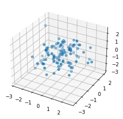
fig = plt.figure()
ax = fig.add_subplot(111, projection='3d')
x = np.random.standard_normal(100)
y = np.random.standard_normal(100)
z = np.random.standard_normal(100)
ax.scatter(x, y, z)
plt.show()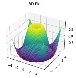
Example with synthetic data
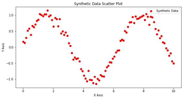
To show Matplotlib in use, let's create a synthetic data set and visualize it with different plot types.
import numpy as np
import matplotlib.pyplot as plt

# Generating synthetic data
np.random.seed(0)
x = np.linspace(0, 10, 100)
y = np.sin(x) + np.random.normal(0, 0.1, 100)
# Line plot
plt.figure(figsize=(10, 5))
plt.plot(x, y, label='Synthetic Data')
plt.xlabel('X Axis')
plt.ylabel('Y Axis')
plt.title('Synthetic Data Line Plot')
plt.legend()
plt.show()
# Scatter plot
plt.figure(figsize=(10, 5))
plt.scatter(x, y, label='Synthetic Data', color='red')
plt.xlabel('X Axis')
plt.ylabel('Y Axis')
plt.title('Synthetic Data Scatter Plot')
plt.legend()
plt.show()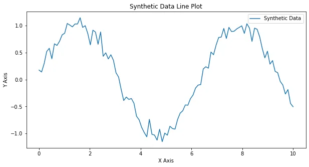
Conclusion
Matplotlib is a powerful and flexible tool for data visualization in Python. In this article we created line plots, bar charts, scatter plots, histograms, pie charts and more. We also customized plots and built advanced visualizations: annotated plots, subplots, logarithmic plots and 3D plots. Using Matplotlib's wide range of features, you can sharpen your visualization skills and present your data clearly and convincingly.
References
- Hunter, J. D. (2007). Matplotlib: A 2D Graphics Environment. Computing in Science & Engineering, 9(3), 90–95.
- Matplotlib documentation: matplotlib.org
- Waskom, M. et al. (2021). Seaborn: Statistical Data Visualization. Journal of Open Source Software, 6(60), 3021. seaborn.pydata.org