

What Is an Imbalanced Data Set, and How Do You Deal with It?
Written by Yasin TANIŞ

What an imbalanced data set is
You build a classification model for a business and it scores 95% accuracy. Everything looks fine. The model goes into use, and soon someone notices it always predicts the same class. Looking at the data again, you find that the class it never detects makes up only 5% of the data. The model's failure comes from an imbalanced data set.
Imbalanced data sets appear in classification problems when the classes are far from evenly distributed. The problem is that the majority class drowns out the minority class: the model leans towards the majority and classifies the minority badly.
When we face imbalanced data, these are the methods we can use to observe correctly and restore balance:
- Choosing the right metrics: precision, recall, F1 score, the ROC curve and AUC
- Resampling: oversampling (random and SMOTE) and undersampling (random, NearMiss, Tomek links, cluster centroids)
- Collecting more data
- Using the
class_weightparameter of classification models so the model learns equally from minority and majority classes - Looking at the performance of other models rather than relying on one
- Taking a different approach, such as anomaly or change detection
First we examine the Credit Card Fraud Detection data set, which is imbalanced, and then we apply several methods to deal with that imbalance.
Examining the data set
Detecting fraud matters to credit card companies: they do not want customers charged for purchases they did not make.
Data set: creditcard.csv (Kaggle)
We want to use this data set to build a model that detects fraudulent transactions. The data comes from card transactions made in Europe in September 2013; each transaction is labelled 1 if it is fraud and 0 if not. For privacy reasons there is little background information, and all variables except Time and Amount have been transformed with PCA (principal component analysis).
Time: seconds elapsed between the first transaction and each transactionAmount: the transaction amount
First we read the data, check for missing values and look at the distribution of the Class variable. Then we standardize Amount and Time, split the data with a hold-out set and build a classification model with logistic regression. We will work with a single model.
# Gerekli kütüphaneler
import pandas as pd
import numpy as np
from sklearn.preprocessing import RobustScaler
from sklearn.linear_model import LogisticRegression
from sklearn.model_selection import train_test_split
from sklearn.metrics import accuracy_score
from sklearn.metrics import confusion_matrix, classification_report,f1_score,recall_score,roc_auc_score, roc_curve
import matplotlib.pyplot as plt
import seaborn as sns
from matplotlib import rc,rcParams
import itertools

import warnings
warnings.filterwarnings("ignore", category=DeprecationWarning)
warnings.filterwarnings("ignore", category=FutureWarning)
warnings.filterwarnings("ignore", category=UserWarning)
# Veri setinin okutulması
df = pd.read_csv("creditcard.csv")
df.head()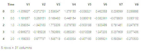
# Veri setindeki değişken ve gözlem sayısı
print("Gözlem sayısı : " ,len(df))
print("Değişken sayısı : ", len(df.columns))
Gözlem sayısı : 284807
Değişken sayısı : 31(The code prints its labels in Turkish: number of observations and number of variables.)
# veri setindeki değişkenlerin tiplerini ve boş değer içerip içermediğini gözlemlemek istiyoruz
df.info()
<class 'pandas.core.frame.DataFrame'>
RangeIndex: 284807 entries, 0 to 284806
Data columns (total 31 columns):
# Column Non-Null Count Dtype
--- ------ -------------- -----
0 Time 284807 non-null float64
1 V1 284807 non-null float64
2 V2 284807 non-null float64
3 V3 284807 non-null float64
4 V4 284807 non-null float64
5 V5 284807 non-null float64
6 V6 284807 non-null float64
7 V7 284807 non-null float64
8 V8 284807 non-null float64
9 V9 284807 non-null float64
10 V10 284807 non-null float64
11 V11 284807 non-null float64
12 V12 284807 non-null float64
13 V13 284807 non-null float64
14 V14 284807 non-null float64
15 V15 284807 non-null float64
16 V16 284807 non-null float64
17 V17 284807 non-null float64
18 V18 284807 non-null float64
19 V19 284807 non-null float64
20 V20 284807 non-null float64
21 V21 284807 non-null float64
22 V22 284807 non-null float64
23 V23 284807 non-null float64
24 V24 284807 non-null float64
25 V25 284807 non-null float64
26 V26 284807 non-null float64
27 V27 284807 non-null float64
28 V28 284807 non-null float64
29 Amount 284807 non-null float64
30 Class 284807 non-null int64
dtypes: float64(30), int64(1)
memory usage: 67.4 MB# 1 sınıfının veri setinde bulunma oranı %0.2, 0 sınıfının ise %99.8
f, ax = plt.subplots(1, 2, figsize=(18, 8))
# Sınıf dağılımı
class_counts = df['Class'].value_counts().sort_values(ascending=False)
# Sınıf sayısına göre patlamayı belirleyin
explode = [0.1] * len(class_counts)
# Sınıf dağılımı için pasta grafik
ax[0].pie(class_counts, labels=class_counts.index, autopct='%1.1f%%', explode=explode, shadow=True)
ax[0].set_title('Dağılım')
ax[0].set_ylabel('')
# Sınıf dağılımı için sayım grafiği (seaborn kullanarak)
sns.countplot(x='Class', data=df, ax=ax[1])
ax[1].set_title('Sınıf Sayısı')
plt.show()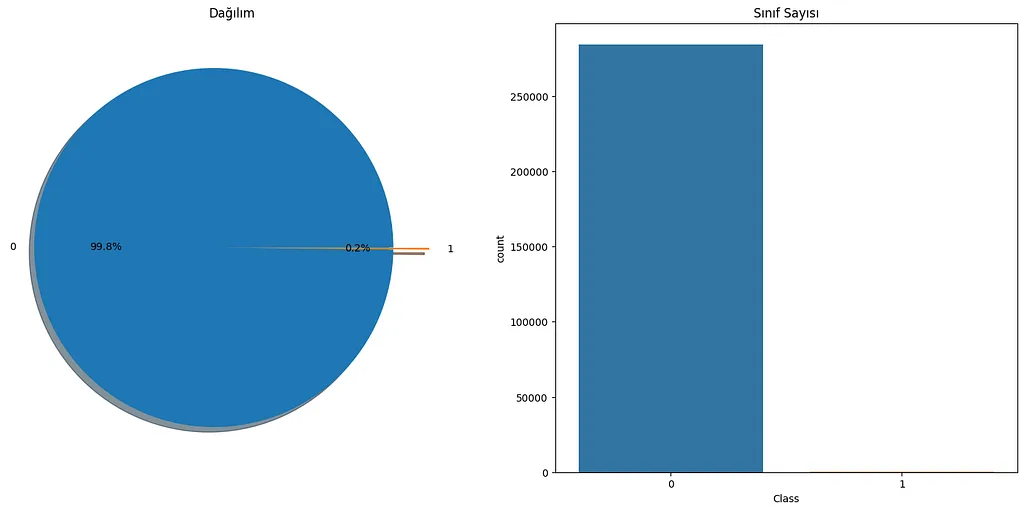
# Time ve Amount değişkenlerini standartlaştırma
rob_scaler = RobustScaler()
df['Amount'] = rob_scaler.fit_transform(df['Amount'].values.reshape(-1,1))
df['Time'] = rob_scaler.fit_transform(df['Time'].values.reshape(-1,1))
df.head()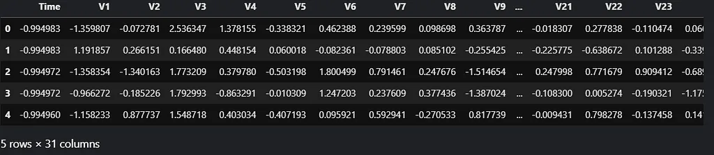
# Hold out yöntemi uygulayıp veri setini eğitim ve test olarak ikiye ayırıyoruz.(%80,%20)
X = df.drop("Class", axis=1)
y = df["Class"]
X_train, X_test, y_train, y_test = train_test_split(X, y, test_size=0.20, random_state=123456)
# modelin tanımlanıp, eğitilmesi ve başarı skoru
model = LogisticRegression(random_state=123456)
model.fit(X_train, y_train)
y_pred = model.predict(X_test)
accuracy = accuracy_score(y_test, y_pred)
print("Accuracy: %.3f"%(accuracy))Accuracy: 0.999Accuracy is the share of correct predictions among all predictions. Our model scores 0.999. We could say it works perfectly, couldn't we? Let's look at the confusion matrix as well.
The confusion matrix
A confusion matrix is a table that summarizes how a classification model performs on test data. It contains the four combinations of predicted and actual values. Here we treat fraud as the positive class:
- True positive (TP): predicted positive, and correct.
- True negative (TN): predicted negative, and correct.
- False positive (FP): predicted positive, but wrong.
- False negative (FN): predicted negative, but wrong.
def plot_confusion_matrix(cm, classes,
                          title='Confusion matrix',
                          cmap=plt.cm.Blues):

    plt.rcParams.update({'font.size': 19})
    plt.imshow(cm, interpolation='nearest', cmap=cmap)
    plt.title(title,fontdict={'size':'16'})
    plt.colorbar()
    tick_marks = np.arange(len(classes))
    plt.xticks(tick_marks, classes, rotation=45,fontsize=12,color="blue")
    plt.yticks(tick_marks, classes,fontsize=12,color="blue")
    rc('font', weight='bold')
    fmt = '.1f'
    thresh = cm.max()
    for i, j in itertools.product(range(cm.shape[0]), range(cm.shape[1])):
        plt.text(j, i, format(cm[i, j], fmt),
                 horizontalalignment="center",
                 color="red")

    plt.ylabel('True label',fontdict={'size':'16'})
    plt.xlabel('Predicted label',fontdict={'size':'16'})
    plt.tight_layout()

plot_confusion_matrix(confusion_matrix(y_test, y_pred=y_pred), classes=['Non Fraud','Fraud'],
                      title='Confusion matrix')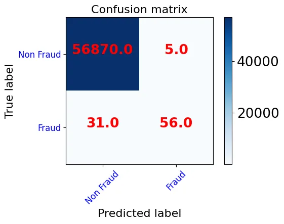
- Of the 56875 transactions that are actually normal, 56870 are predicted correctly and 5 are wrongly flagged as fraud (FP).
- Of the 87 transactions that are actually fraud, 56 are caught (TP) and 31 are missed (FN).
The model claims 0.999 accuracy, but the confusion matrix shows a high error rate in the fraud class. The model predicts the majority class well and the minority class poorly. Because there are so many more normal transactions than fraudulent ones, the model looks successful by predicting the normal class.
The lesson: accuracy is not a good performance measure for classification models, especially when the data is as imbalanced as ours. Let's look at how to deal with the imbalance, which methods to apply and which metrics to measure performance with.
Choosing the right metrics
We have seen that accuracy is not enough; we need other metrics to measure performance.
Precision: the share of predicted positives that are actually positive. Low precision means many false positives. Precision = TP / (TP + FP).
Recall: the share of actual positives that we predicted as positive. Low recall means many false negatives; it should be as high as possible. Recall = TP / (TP + FN).
F1 score: it is hard to compare a model with low precision and high recall against one with the opposite. The F1 score measures both together as the harmonic mean of precision and recall. F1 = 2 × (Precision × Recall) / (Precision + Recall).
Let's look at these metrics for our model. The classification report shows the main metrics per class.
#sınıflandırma raporu
print(classification_report(y_test, y_pred))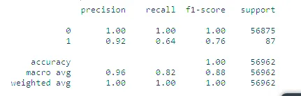
Precision per class:
- Class 0 (normal): 56870 + 31 = 56901 transactions predicted normal, 56870 of them correctly. Precision ≈ 1.00 (56870 / 56901).
- Class 1 (fraud): 5 + 56 = 61 transactions predicted fraud, 56 of them correctly. Precision ≈ 0.92 (56 / 61).
Recall per class:
- Class 0 (normal): of 56870 + 5 = 56875 normal transactions, 56870 are predicted correctly. Recall ≈ 1.00.
- Class 1 (fraud): of 31 + 56 = 87 fraudulent transactions, 56 are predicted correctly. Recall = 56 / 87 ≈ 0.64.
The recall values make the failure on class 1 plain to see. The F1 score is the harmonic mean of recall and precision. Support is the actual number of examples in each class; the gap between the classes shows a structural weakness of the measurements, since the imbalance itself affects them.
The ROC curve
The ROC curve is a chart of a classification model's performance across all decision thresholds. It plots two values:
- True positive rate (TPR), which is recall: TPR = TP / (TP + FN)
- False positive rate (FPR), the rate of false alarms on normal transactions: FPR = FP / (FP + TN)
The curve plots TPR against FPR at different thresholds; it starts at (0,0) and ends at (1,1). A good model produces a curve that rises quickly from 0 to 1.
AUC (area under the ROC curve)
AUC sums up the ROC curve in one number: it measures the whole area under the curve from (0,0) to (1,1). The best value is 1; random guessing gives 0.5.
# Auc Roc Curve
def generate_auc_roc_curve(clf, X_test):
    y_pred_proba = clf.predict_proba(X_test)[:, 1]
    fpr, tpr, thresholds = roc_curve(y_test,  y_pred_proba)
    auc = roc_auc_score(y_test, y_pred_proba)
    plt.plot(fpr,tpr)
    plt.show()
    pass

generate_auc_roc_curve(model, X_test)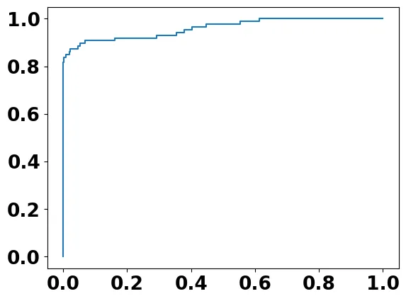
y_pred_proba = model.predict_proba(X_test)[:, 1]
auc = roc_auc_score(y_test, y_pred_proba)
print("AUC ROC Curve with Area Under the curve = %.3f"%auc)
AUC ROC Curve with Area Under the curve = 0.961Note: AUC evaluates overall classification performance. Because it gives no more weight to one class than the other, it does not reflect performance on the minority class well.
Now let's apply several methods to the data set to remove the imbalance.
Important: these methods must be applied to the training set only. Applied to the test set, they make a correct evaluation impossible.
Resampling
Resampling makes a data set more balanced by adding new examples to the minority class or removing examples from the majority class. Undersampling drops majority examples; oversampling multiplies minority examples.
Oversampling
Oversampling balances the data by duplicating examples of the minority class.
Random oversampling:
- Randomly chosen minority examples are added to balance the data set.
- It can be used when the data set is small.
- It can lead to overfitting.
RandomOverSampler takes a sampling_strategy argument. With sampling_strategy='minority' the minority class is multiplied until it matches the majority class. The argument also accepts a decimal: if the majority class has 1000 examples and the minority 100, sampling_strategy=0.5 raises the minority to 500.
# random oversampling önce eğitim setindeki sınıf sayısı
y_train.value_counts()
0 227440
1 405
Name: Class, dtype: int64# RandomOver Sampling uygulanması (Eğitim setine uygulanıyor)
from imblearn.over_sampling import RandomOverSampler
oversample = RandomOverSampler(sampling_strategy='minority')
X_randomover, y_randomover = oversample.fit_resample(X_train, y_train)# random oversampling den sonra eğitim setinin sınıf sayısı
y_randomover.value_counts()1 227440
0 227440
Name: Class, dtype: int64# modelin eğitilmesi ve başarı oranı
model.fit(X_randomover, y_randomover)
y_pred = model.predict(X_test)
accuracy = accuracy_score(y_test, y_pred)
print("Accuracy: %.3f%%" % (accuracy))Accuracy: 0.977plot_confusion_matrix(confusion_matrix(y_test, y_pred=y_pred), classes=['Non Fraud','Fraud'],
title='Confusion matrix')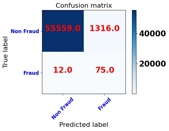
#sınıflandırma raporu
print(classification_report(y_test, y_pred)) precision recall f1-score support
0 1.00 0.98 0.99 56875
1 0.05 0.86 0.10 87
accuracy 0.98 56962
macro avg 0.53 0.92 0.55 56962
weighted avg 1.00 0.98 0.99 56962After random oversampling, the model's accuracy drops to 0.977. The confusion matrix and classification report show that most transactions flagged as fraud are false alarms, which lowers the precision of class 1 to 0.05. In return, the recall of class 1 rises to 0.86: 75 of the 87 frauds are caught. Normal transactions are predicted slightly less well than with the first model, but this jump in catching fraud is a strong reason to prefer the model trained after random oversampling.
SMOTE oversampling:
To avoid overfitting, synthetic minority examples are generated instead of copies:
- A random example is picked from the minority class.
- Its k nearest neighbours are found.
- One neighbour is picked at random; a line segment is drawn in feature space between the example and that neighbour, and the synthetic example is created on that line.
# smote dan önce eğitim setindeki sınıf sayısı
y_train.value_counts()0 227440
1 405
Name: Class, dtype: int64# Smote uygulanması (Eğitim setine uygulanıyor)
from imblearn.over_sampling import SMOTE
oversample = SMOTE()
X_smote, y_smote = oversample.fit_resample(X_train, y_train)# smote dan sonra eğitim setinin sınıf sayısı
y_smote.value_counts()1 227440
0 227440
Name: Class, dtype: int64# modelin eğitilmesi ve başarı oranı
model.fit(X_smote, y_smote)
y_pred = model.predict(X_test)
accuracy = accuracy_score(y_test, y_pred)
print("Accuracy: %.3f%%" % (accuracy))Accuracy: 0.975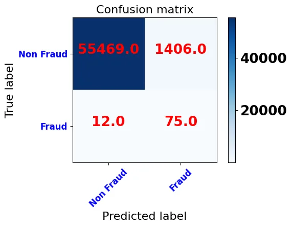
plot_confusion_matrix(confusion_matrix(y_test, y_pred=y_pred), classes=['Non Fraud','Fraud'],
                      title='Confusion matrix')
#sınıflandırma raporu
print(classification_report(y_test, y_pred)) precision recall f1-score support
0 1.00 0.98 0.99 56875
1 0.05 0.86 0.10 87
accuracy 0.98 56962
macro avg 0.53 0.92 0.54 56962
weighted avg 1.00 0.98 0.99 56962The results after SMOTE are similar to random oversampling: again 75 of the 87 frauds are caught, while false alarms rise to 1406.
Undersampling
Undersampling balances the data by removing examples from the majority class and suits large data sets. Our data set is not large enough for it to work well, but we explain the methods and show how some of them are applied.
Random undersampling:
- The examples to remove are chosen at random.
- It can be used if you have a large data set.
- Random selection can lose information.
# random undersampling den önce eğitim setindeki sınıf sayısı
y_train.value_counts()
0 227440
1 405
Name: Class, dtype: int64from imblearn.under_sampling import RandomUnderSampler
# transform the dataset
ranUnSample = RandomUnderSampler()
X_ranUnSample, y_ranUnSample = ranUnSample.fit_resample(X_train, y_train)# Random undersampling sonra
y_ranUnSample.value_counts()1 405
0 405
Name: Class, dtype: int64NearMiss undersampling:
- Reduces information loss.
- Is based on the KNN algorithm.
- Computes the distance from majority examples to minority examples.
- Keeps the majority examples closest to the minority class, according to a given k.
Tomek links: for each pair of nearest examples from different classes, the majority example is removed, which widens the gap between the two classes.
Cluster centroids: unimportant examples are removed from the data set; whether an example matters is decided by clustering.
Undersampling and oversampling can be combined to build more balanced data sets.
Other methods
- Collecting more data
- Using the
class_weightparameter so the model learns equally from minority and majority classes - Looking at the performance of other models, not just one
- Taking a different approach, such as anomaly or change detection
Which method works best depends on the data set at hand. Trying the methods and choosing the one that fits your data gives the best result.
References
- Kaggle: On imbalanced data sets (Yasin Tanış, in Turkish)
- Miuul: What is an imbalanced data set (in Turkish)
- Machine Learning Mastery: Random oversampling and undersampling
- Machine Learning Mastery: SMOTE oversampling
- Towards Data Science: Understanding the confusion matrix
- Towards Data Science: Understanding the AUC-ROC curve
- Machine Learning Mastery: Tactics to combat imbalanced classes